Categories: Statistical Mechanics | Quantum mechanics | Quantum field theory | Probability distributions

Fermi-Dirac statistics

In statistical mechanics, Fermi-Dirac statistics determines the statistical distribution of fermions over the energy states for a system in thermal equilibrium. Fermions are particles which are indistinguishable and obey the Pauli exclusion principle, i.e., that no two particles may occupy the same state at the same time. Statistical thermodynamics is used to describe the behaviour of large numbers of particles. A collection of non-interacting fermions is called a Fermi gas.

Fermi-Dirac (or F-D) statistics are closely related to Maxwell-Boltzmann statistics and Bose-Einstein statistics. While F-D statistics holds for fermions, B-E statistics plays the same role for bosons – the other type of particle found in nature. M-B statistics describes the velocity distribution of particles in a classical gas and represents the classical (high-temperature) limit of both F-D and B-E statistics. M-B statistics are particularly useful for studying gases, and B-E statistics are particularly useful when dealing with photons and other bosons. F-D statistics are most often used for the study of electrons in solids. As such, they form the basis of semiconductor device theory and electronics. The invention of quantum mechanics, when applied through F-D statistics, has made advances such as the transistor possible. For this reason, F-D statistics are well-known not only to physicists, but also to electrical engineers.

F-D statistics was introduced in 1926 by Enrico Fermi and Paul Dirac and applied in 1927 by Arnold Sommerfeld to electrons in metals.

The expected number of particles in an energy state i for F-D statistics is

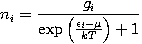
$n_i = \frac{g_i}{\exp\left(\frac{\epsilon_i-\mu}{k T}\right) + 1}$

where:

n_i is the number of particles in state i

g_i is the degeneracy of state i

ε_i is the energy of state i

μ is the chemical potential. Sometimes the Fermi energy E_F is used instead, as a low-temperature approximation.

k is Boltzmann's constant

T is absolute temperature

exp is the exponential function

Derivation of the Fermi-Dirac distribution

Say there are two fermions placed in a system with four energy levels. There are six possible arrangements of such a system, which are shown in the diagram below.

   ε₁   ε₂   ε₃   ε₄
A  *    *
B  *         *
C  *              *
D       *    *
E       *         *
F            *    *

Each of these arrangements is called a microstate of the system. The ergodic hypothesis states that at thermal equilibrium, each of these microstates will be equally likely, subject to the constraints that there be a fixed total energy and a fixed number of particles.

Depending on the values of the energy for each state, it may be that total energy for some of these six combinations is the same as others. Indeed, if we assume that the energies are multiples of some fixed value ε, the energies of each of the microstates become:

A: 3ε
B: 4ε
C: 5ε
D: 5ε
E: 6ε
F: 7ε

So if we know that the system has an energy of 5ε, we can conclude that it will be equally likely that it is in state C or state D. Note that if the particles were distinguishable (the classical case), there would be twelve microstates altogether, rather than six.

Now suppose we have a number of energy levels, labelled by index i , each level having energy ε_i and containing a total of n_i particles. Suppose each level contains g_i distinct sublevels, all of which have the same energy, and which are distinguishable. For example, two particles may have different momenta, in which case they are distinguishable from each other, yet they can still have the same energy. The value of g_i associated with level i is called the "degeneracy" of that energy level. The Pauli exclusion principle states that only one fermion can occupy any such sublevel.

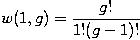
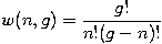
Let w(n,g) be the number of ways of distributing n particles among the g sublevels of an energy level. Its clear that there are g ways of putting one particle into a level with g sublevels, so that w(1,g)=g which we will write as:

$w(1,g)=\frac{g!}{1!(g-1)!}$

We can distribute 2 particles in g sublevels by putting one in the first sublevel and then distributing the remaining n-1 particles in the remaining g-1 sublevels, or we could put one in the second sublevel and then distribute the remaining n-1 particles in the remaining g-2 sublevels, etc. so that w(2,g)=w(1,g-1)+w(1,g-2)+...+w(1,1) or

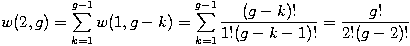
$w(2,g)=\sum_{k=1}^{g-1}w(1,g-k) = \sum_{k=1}^{g-1}\frac{(g-k)!}{1!(g-k-1)!}=\frac{g!}{2!(g-2)!}$

where we have used the following theorem involving binomial coefficients:

$\sum_{k=n}^g \frac{k!}{n!(k-n)!}=\frac{(k+1)!}{(n+1)!(k-n)!}$

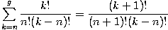
Continuing this process, we can see that w(n,g) is just a binomial coefficient

$w(n,g)=\frac{g!}{n!(g-n)!}$

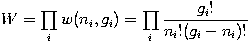
The number of ways that a set of occupation numbers n_i can be realized is the product of the ways that each individual energy level can be populated:

$W = \prod_i w(n_i,g_i) = \prod_i \frac{g_i!}{n_i!(g_i-n_i)!}$

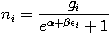
Following the same procedure used in deriving the Maxwell-Boltzmann distribution, we wish to find the set of n_i for which W is maximised, subject to the constraint that there be a fixed number of particles, and a fixed energy. We constrain our solution using Lagrange multipliers forming the function:

$f(n_i)=\ln(W)-\alpha(N-\sum n_i)+\beta(E-\sum n_i \epsilon_i)$

Taking the derivative with respect to n_i and setting the result to zero and solving for n_i yields the Fermi-Dirac population numbers:

$n_i = \frac{g_i}{e^{\alpha+\beta \epsilon_i}+1}$

It can be shown thermodynamically that β=1/kT where k is Boltzmann's constant and T is the temperature. The term containing α is variously written:

$\left.\right. e^\alpha = e^{-\mu/kT} = 1/z$

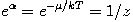
where μ is the chemical potential and z is the absolute activity.

Encyclopedia

Dictionary

Quotes

Fermi-Dirac statistics

Derivation of the Fermi-Dirac distribution

See Also

The Online Encyclopedia and Dictionary

Encyclopedia

Dictionary

Quotes

Fermi-Dirac statistics

Derivation of the Fermi-Dirac distribution

See Also